1-15: Nested loops and Matrices
0.1 To-Do
1 Purpose
embedded for loops
functions within a script
using matrices
named values in a vector
2 Questions about the material…
The files for this lesson:
- Script (only one this lesson): you can download the script here
If you have any questions about the material in this lesson, feel free to email them to the instructor, Charlie Belinsky, at belinsky@msu.edu.
3 Functions within a script
In the previous two lessons, we created a separate script for the functions used in the lesson. For this lesson, the function isPrime3() has been put inside the main script. It is not usually best practice to put functions inside the calling script (why this is true is an application question). However, there are many occasions where you will see functions put directly inside a script, so it is good to be familiar with this practice.
3.1 functions need to be declared
Functions are like variables in that they store information to a named objects – and objects must be declared before they are used. If you are going to code a function directly in the script that calls the function then you need to declare the function before you call the function.
4 Nesting for loops: isPrime3()
In the previous lesson’s function script, the function isPrime2(), has a for loop that cycles through all of the possible divisors for the dividend given by the caller. If none of the modulus calculations are zero (i.e., every division has a remainder), then we know the dividend is prime. isPrime3() extends isPrime2() so that it can check multiple dividends for prime instead of one.
This means we need nested for loops (for loops inside of for loops). The outer for loop cycles through each of the dividends and the inner for loop cycles though all the possible divisors for the specific dividend:
for(each dividend we want to check)         # outer loop
{
  for(each divisor of the current dividend) # inner loop
  {

  }
}
4.1 Examples of isPrime3()
Before we look at the code, let’s look at an example of its use:
primeTest1 = isPrime3(c(12,13,14,15,16,17));In the Environment, primeTest1, which stored the return value, is called a Named logi.
primeTest1: Named logi [1:6] FALSE TRUE FALSE FALSE FALSE TRUElogi means the vector values are Boolean and Named means the individual vector values are named. You cannot see the names in the Environment but you can in the Console:
> primeTest1
   12    13    14    15    16    17
FALSE  TRUE FALSE FALSE FALSE  TRUE
The names are the same as the dividend values passed in by the caller. How this is done will be shown later in this lesson.
One advantage to Named variables is that you can index the vector by either name or position:
> primeTest1["14"]
   14
FALSE
> primeTest1[3]
   14
FALSE
5 Nested for loops
isPrime3() has two for loops:
outer loop: indexes through the range of dividends supplied by the caller
inner loop: indexes through the range of divisors that will be used to check the dividend for prime
- like last lesson, the range will be from 2 to one less than the dividend
5.1 Outer loop
The job of the outer loop is cycle through each dividends. The index value, i, determines the current dividend, indexed from the dividends vector. The current dividend gets used inside the inner for loop.
In the example above (Section 4.1),
primeNum[1] = 12;
primeNum[2] = 13;
…
primeNum[6] = 17;
  «for(i in 1:length(dividends))»
  {
    primeNum[i] = TRUE;

    for(j in 2:(dividends[«i»]-1))
    {
      if(dividends[«i»] %% j == 0)
      {
        primeNum[«i»] = FALSE;
      }
    }
  «}»
5.2 Inner loop
isPrime2() uses a for loop to check all the possible divisors for the dividend. That for loop is now the inner for loop in isPrime3(). The inner for loop cycles through every single value from 2 to one less that the current dividend, except the index variable is now j, because i was used by the outer loop.
  for(i in 1:length(dividends))
  {
     primeNum[i] = TRUE;

    «for(j in 2:(dividends[i]-1))»  # 2 to one less than current dividend
    «{»
      if(dividends[i] %% «j» == 0)
      {
        primeNum[i] = FALSE;
      }
    «}»
  }
The return value needs to specify if each dividend is prime (TRUE) or not (FALSE). This means a vector of Boolean values needs to be set and returned to the caller so the return vector returned has the same number of values as the vector dividends.
5.3 Set up the return value
The function returns a Boolean vector to the caller that is the same length as dividends passed in by the caller. The return vector is created in the first line of the function:
primeNum = c();Like before, we assume that the dividend is prime until proven otherwise, so at the beginning of the outer for loop, we set the current primeNum to TRUE:
primeNum[i] = TRUE;The inner for loop goes through all possible divisors. If one of the divisors divides the dividend evenly then the dividend is not prime and then switches the single value in the vector primeNum to FALSE.
primeNum[i] = FALSE;isPrime3 = function(dividends)
{
«primeNum = c();»
for(i in 1:length(dividends)) # outer loop
{
«primeNum[i] = TRUE;» # default is that dividend is prime
for(j in 2:(dividends[i]-1)) # inner loop
{
if(dividends[i] %% j == 0) # i from outer loop indexing dividends
{
«primeNum[i] = FALSE;» # dividend not be prime
}
}
}
names(primeNum) = dividends;
«return(primeNum);»
}5.4 Return named vector
If we just returned primeNum to the caller, the return would be a Boolean vector that can be indexed by position only.
It order to make the return value more readable to the caller, we attached names to each vector value. Since the caller want to know the prime status of each dividend, it makes sense to name the return with the dividend values:
names(primeNum) = dividends;In the end, we return primeNum back to the caller and primeNum gets save to the variable the caller set equal to the function:
return(primeNum);5.5 Console Examples
We can call the function isPrime3() from within the script, as before (Section 4.1), or from the Console:
> isPrime3(30:39)
   30    31    32    33    34    35    36    37    38    39
FALSE  TRUE FALSE FALSE FALSE FALSE FALSE  TRUE FALSE FALSE
> isPrime3(seq(from=17, to=57, by=10))
   17    27    37    47    57
 TRUE FALSE  TRUE  TRUE FALSE
If names(primeNum) = dividends; was taken out of the function then the return values would look like this:
> isPrime3(30:39)
 [1] FALSE  TRUE FALSE FALSE FALSE FALSE FALSE  TRUE FALSE FALSE
> isPrime3(seq(from=17, to=57, by=10))
[1]  TRUE FALSE  TRUE  TRUE FALSE
6 Two-dimensional vectors
One of the more natural uses of nested for loops in R is the creation of two-dimensional vectors, also called a matrix.
6.1 What is a matrix
A matrix is somewhat of a cross between a vector and a data frame. A matrix has rows and columns like a data frame. However, like a vector, all values in a matrix are of the same type. This means that calculations on a matrix can be applied to all values as opposed to just one column. We will talk more about the use of matrices in a later lesson.
6.2 Matrix creation
Just like c() is used to create a vector, matrix() isused to create a matrix, with the arguments nrow and ncol giving the dimensions of the matrix.
We can create an empty matrix:
> matrix(nrow=4, ncol=3)
     [,1] [,2] [,3]
[1,]   NA   NA   NA
[2,]   NA   NA   NA
[3,]   NA   NA   NA
[4,]   NA   NA   NA
Or fill the matrix with values:
> matrix(data=1:12, nrow=4, ncol=3)
     [,1] [,2] [,3]
[1,]    1    5    9
[2,]    2    6   10
[3,]    3    7   11
[4,]    4    8   12
6.3 Subsetting a matrix
Let’s save the matrix as the variable, testMatrix, so that we can use the matrix:
> testMatrix = matrix(data=1:12, nrow=4, ncol=3)To get a specific value from the matrix, you need two values, a row and a column:
> testMatrix[1,2]
[1] 5
> testMatrix[3,1]
[1] 3
> testMatrix[4,3]
[1] 12
You can get a whole row by leaving the column blank and a whole column by leaving the row blank:
> testMatrix[3,]
[1] 3  7 11
> testMatrix[,2]
[1] 5 6 7 8
6.4 Matrices are often all combinations of two factors
One common use of a matrix is to create a table the contains every combination of two factors. For instance, we can have a vector of temperature values and a vector of humidity values and create a heat index matrix for every temperature/humidity combination:
7 Multiplication table
We will start with a simpler example: a multiplication table. For this table we will have two numeric vectors and populate the matrix with every possible multiplication between values in the two vectors:
| 1 | 2 | 3 | |
|---|---|---|---|
| 1 | 1 | 2 | 3 |
| 2 | 2 | 4 | 6 |
| 3 | 3 | 6 | 9 |
| 4 | 4 | 8 | 12 |
| 5 | 5 | 10 | 15 |
7.1 Setting up the matrix
First we need our numeric vectors:
### Factors for multiplication table
mult1 = 2:6;
mult2 = 8:10;
Then we need to create an empty matrix that has the correct number of rows and columns – given by the lengths of mult1 and mult2:
### Create a matrix that will contain the calculations
multTable = matrix(nrow=length(mult1),
                   ncol=length(mult2));
7.2 Using nested for loops to fill matrix
We use nested for loops to cycle through every possible combination of mult1 and mult2.
The outer loop cycles through mult1 and the inner loop cycles through mult2:
for(i in 1:length(mult1))   # outer loop (for each mult1)
{
  for(j in 1:length(mult2)) # inner loop (for each mult2)
  {
    # The [i,j] cell get set to the multiplication of the corresponding i and j values
    multTable[i,j] = mult1[i] * mult2[j];
  }
}
The calculations go in this order:
2*8, 2*9, 2*10, 3*8, 3*9, 3*10, 4*8, 4*9, 4*10, 5*8, 5*9, 5*10, 6*8, 6*9, 6*10.
Aside from cycling through values, the only code is this line:
multTable[i,j] = mult1[i] * mult2[j]; multTable is a 2D matrix and needs 2 values to subset it (i and j). The [i, j] spot in the matrix gets populated the ith value of mult1 multiplied by the jth value of mult2.
7.3 Naming rows and columns
After we execute the for loop, we have a matrix that looks like this:
> multTable
     [,1] [,2] [,3]
[1,]   16   18   20
[2,]   24   27   30
[3,]   32   36   40
[4,]   40   45   50
[5,]   48   54   60
Let’s make the matrix more visually informative by naming the rows and columns to the values in mult1 and mult2:
rownames(multTable) = mult1;
colnames(multTable) = mult2;
Now we get something that’s easier to read:
> multTable
   8  9 10
2 16 18 20
3 24 27 30
4 32 36 40
5 40 45 50
6 48 54 60and can use the names to refer to rows and columns:
> multTable["4", "10"]
[1] 40
> multTable["2", "9"]
[1] 18
7.4 Indexing named numeric values
Rownames and column names are always characters – this is why the values are in quotes. Numeric value are used to index rows and columns.
multTable[4, 10]is the value in row 4 and column 10, which does not exist so this would be an error.multTable["4", "10"]is the value in the row named “4” and column named “10”
8 Wind Chill Matrix
We will do a slightly more complicated matrix that combines temperature values and wind speed values to create a wind chill matrix
8.1 Matrix setup
We first need our temperature and wind speed values. This time we will use sequences that gives every 10th value:
temps = seq(from=40, to=-20, by=-10); # 40, 30, 20...
speeds = seq(from=5, to=45, by=10);   # 5, 15, 25 ...
And create a matrix that has the correct number of rows and columns based on the length of temps and speeds:
windChillTable = matrix(nrow=length(temps),
                        ncol=length(speeds));
Finally, we will add row names and column names to make the matrix easier to read:
rownames(windChillTable) = temps;
colnames(windChillTable) = speeds;
8.2 changing index names in nested for loops
It is common programming practice to use i and j for the index values of the outer and inner for loops, respectively. However, this is often not the most intuitive naming. For this example I will use row and col as the index values:
for(«row» in 1:length(temps))     # cycle thru temps for each row
{
  for(«col» in 1:length(speeds))  # cycle thru speeds for each column
  {
    windChillTable[row,col] = 35.74 +
                              0.6215*temps[row] -
                              35.75*(speeds[col]^0.16) +
                              0.4275*temps[row]*(speeds[col]^0.16);
  }
}
8.3 Populating the matrix
The windChillTable for loop operates almost exactly the same as the multiplication table. It has a outer loop the cycles through one set of values (temperatures) and send each temperature into the inner loop where it cycles through the second set of values (wind speeds). The main difference is the formula, supplied by the National Weather Service, is more complicated.
But, like the multiplication matrix, each cell in the wind chill matrix…
windChillMatrix[row,col]is set to a formula that contains the current temperature:
    windChillTable[row,col] = 35.74 +
                              0.6215*«temps[row]» -
                              35.75*(speeds[col]^0.16) +
                              0.4275*«temps[row]»*(speeds[col]^0.16);
and the current wind speed:
    windChillTable[row,col] = 35.74 +
                              0.6215*temps[row] -
                              35.75*(«speeds[col]»^0.16) +
                              0.4275*temps[row]*(«speeds[col]»^0.16);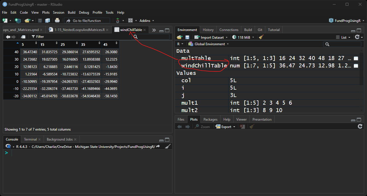
9 Application
1) For this application, all functions, code, and answers to questions will go in one script named 1-15.r. Make sure you test all code thoroughly in your script.
2) In comments answer:
What is the disadvantage of putting a function in the same script that it is called from?
How many times does the inner for loop get executed in windChillTable() in Section 8.1?
If you reverse the order of the for loop in the multiplication matrix in Section 7.2 (i.e., outer loop cycles through mult2, inner loop cycles through mult1), what is the order of the calculations?
3) Reverse the order of the for loops in the wind chill matrix so that the rows are wind speeds and columns and temperatures.
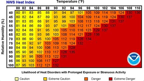
4) Using nested for loops, create a heat index matrix
- The formula for heat index is on page 2 of this document
- The formula is only meaningful for temperatures from 70-100 (F) and humidity from 40-80 (percent)
- You can round the numbers to two significant digits
- 5.12x10⁻⁷ can be coded as 5.12e-7
5) Create a wind chill matrix function that has temperature and wind speed as arguments and the return value is the wind chill matrix.
So, this code:
windChill = windchill(temps = seq(from=40, to=-20, by=-10),
                      speeds = seq(from=5, to=45, by=10))
should save to windChill a matrix that looks like this Figure 2
6) Challenge: Create a function that takes a vector of numbers as an argument and returns every pair where one number evenly divides another number.
So, if you have the vector
c(3,4,7,12,14,15)- you have four pairs: (1) 3 divides 12, (2) 4 divides 12, (3) 7 divides 14, (4) 3 divides 15
- Do not include pairs with the same number (e.g., 3 divides 3, 14 divides 14)
the answer should a named vector and look like this – the order of the pairs does not matter:
> evenlyDivides( c(3,4,7,12,14,15) )
 3   4  7  3
12 12 14 15- A good middle step is to print something to the Console every time you get a pair where one divides the other.
- Info about naming individual values: Extension: Create and modify Named vectors
Save the script as app1-15.r in your scripts folder and email your Project Folder to Charlie Belinsky at belinsky@msu.edu.
Instructions for zipping the Project Folder are here.
If you have any questions regarding this application, feel free to email them to Charlie Belinsky at belinsky@msu.edu.
9.1 Questions to answer
Answer the following in comments inside your application script:
What was your level of comfort with the lesson/application?
What areas of the lesson/application confused or still confuses you?
What are some things you would like to know more about that is related to, but not covered in, this lesson?
10 Extension: Create and modify Named vectors
You can manually create a named vector in the Console:
> myVec = c(1,2,3,4)
> names(myVec) = c("z", "y", "x", "w")
> myVec
z y x w
1 2 3 4
names() can also be used to modify the names of individual values in a vector:
> names(myVec)[2] = "q"
> myVec
z «q» x w
1 2 3 4